Hyperparameter Selection¶

ivis uses several hyperparameters that can have an impact on the desired embeddings:

embedding_dims: Number of dimensions in the embedding space.
k: The number of nearest neighbours to retrieve for each point.
n_epochs_without_progress: After n number of epochs without an improvement to the loss, terminate training early.
model: the keras model that is trained using triplet loss. If a model object is provided, an embedding layer of size embedding_dims will be appended to the end of the network. If a string is provided, a pre-defined network by that name will be used. Possible options are: ‘szubert’, ‘hinton’, ‘maaten’. By default the ‘szubert’ network will be created, which is a selu network composed of 3 dense layers of 128 neurons each, followed by an embedding layer of size ‘embedding_dims’.

k , n_epochs_without_progress, and model are tunable parameters that should be selected on the basis of dataset size and complexity. The following table summarizes our findings:

Observations	`k`	`n_epochs_without_progress`	`model`
< 1000	10-15	20-30	maaten
1000-10000	10-30	10-20	maaten
10000-50000	15-150	10-20	maaten
50K-100K	15-150	10-15	maaten
100K-500K	15-150	5-10	maaten
500K-1M	15-150	3-5	szubert
> 1M	15-150	2-3	szubert

We will now look at each of these parameters in turn.

`k`¶

This parameter controls the balance between local and global features of the dataset. Low k values will result in prioritisation of local dataset features and the overall global structure may be missed. Conversely, high k values will force ivis to look at broader aspects of the data, losing desired granularity. We can visualise effects of low and large values on k on the Levine dataset (104,184 x 32).

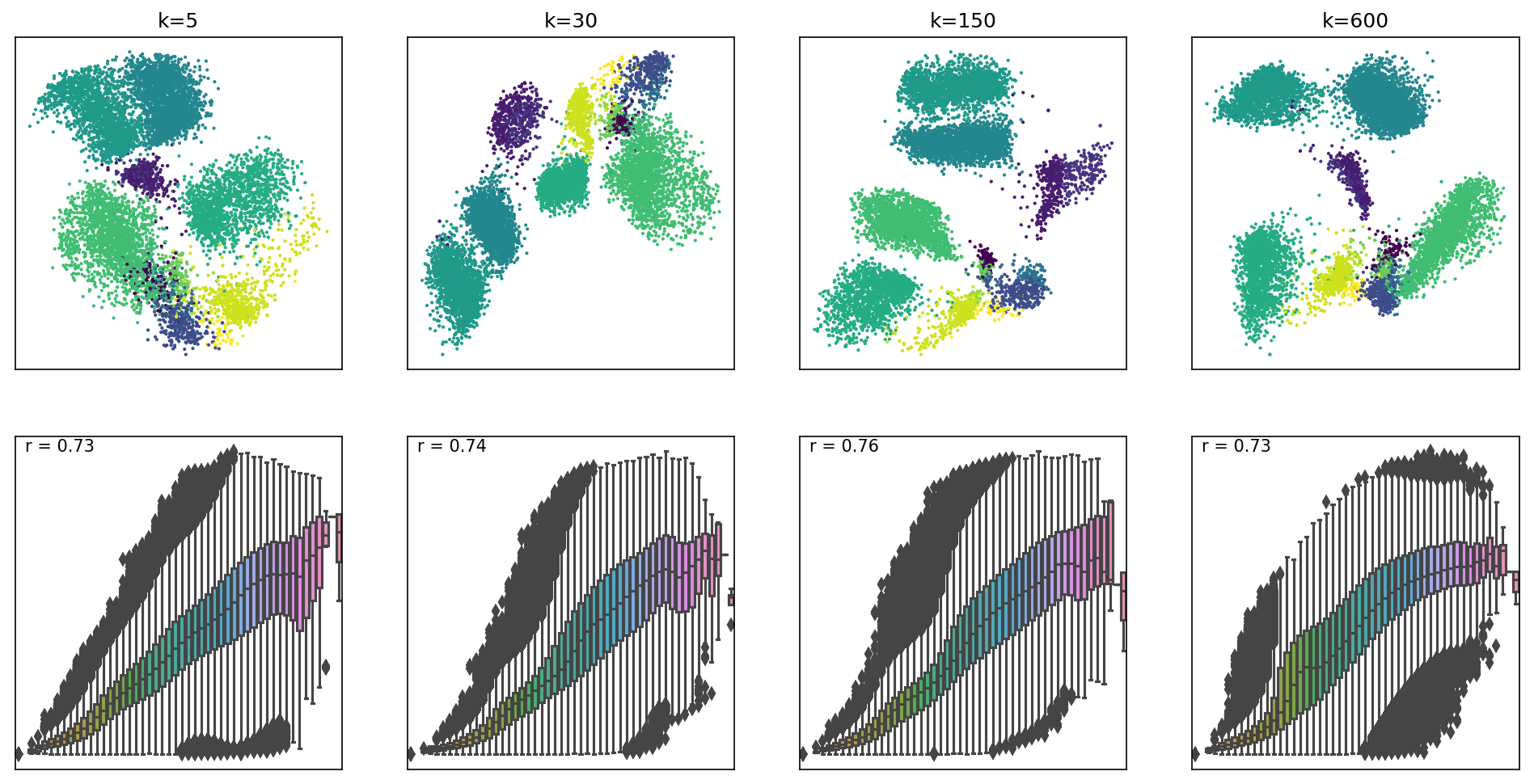
Box plots represent distances across pairs of points in the embeddings, binned using 50 equal-width bins over the pairwise distances in the original space using 10,000 randomly selected points, leading to 49,995,000 pairs of pairwise distances. For each embedding, the value of the Pearson correlation coefficient computed over the pairs of pairwise distances is reported. We can see that where k=5, smaller distances are better preserved, whilst larger distances have higher variability in the embedding space. As k values increase, larger distances are beginning to be better preserved as well. However, for very large k, smaller distances are no longer preserved.

To establish an appropriate value of k, we evaluated a range of values across a severao subsamples of varying sizes, keeping n_epochs_without_progress and model hyperparameters fixed.

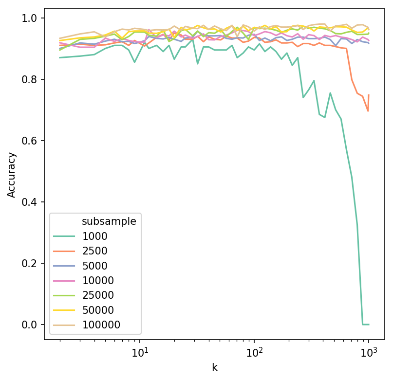
Accuracy was calculated by training a Support Vector Machine classifier on 75% of each subsample and evaluating the classifier performance on the remaining 25%, whilst predicting manually assigned cell types in the Levine dataset. Accuracy was high and generally stable for k between 10 and 150. A decrease was observed when k was considerably large in relation to subsample size.

Overall, ivis is fairly robust to values of k, which can control the local vs. global trade off in the embedding space.

`n_epochs_without_progress`¶

This patience hyperparameter impacts both the quality of embeddings and speed with which they are generated. Generally, the higher n_epochs_without_progress are, the more accurate are the low-dimensional features. However, this comes at a computational cost. Here we examine, the speed vs. accuracy trade-off and recommend sensible defaults. For this experiment ivis hyperparameters were set to k=15 and model='maaten'.

Three datasets were used Levine (104,184 x 32), MNIST (70,000 x 784), and Melanoma (4,645 x 23,686). The Melanoma featurespace was further reduced to n=50 using Principal Component Analysis.

For each dataset, we trained a Support Vector Machine classifier to assess how well ivis embeddings capture manually supplied response variable information. For example, in case of an MNIST dataset, the response variable is the digit label, whilst for Levine and Melanoma datasets it is the cell type. SVM classifier was trained on ivis embeddings representing 3%, 40%, and 95% of the data obtained using a stratified random subsampling. The classifier was then validated on the ivis embeddings of the remaining 97%, 60%, and 5% of data. For each training set split, an ivis model was trained by keeping the k and model hyperparameters constat, whilst varying n_epochs_without_progress. Finally, classification accuracies were noramlised to a 0-1 range to facilitate comparisons between datasets.

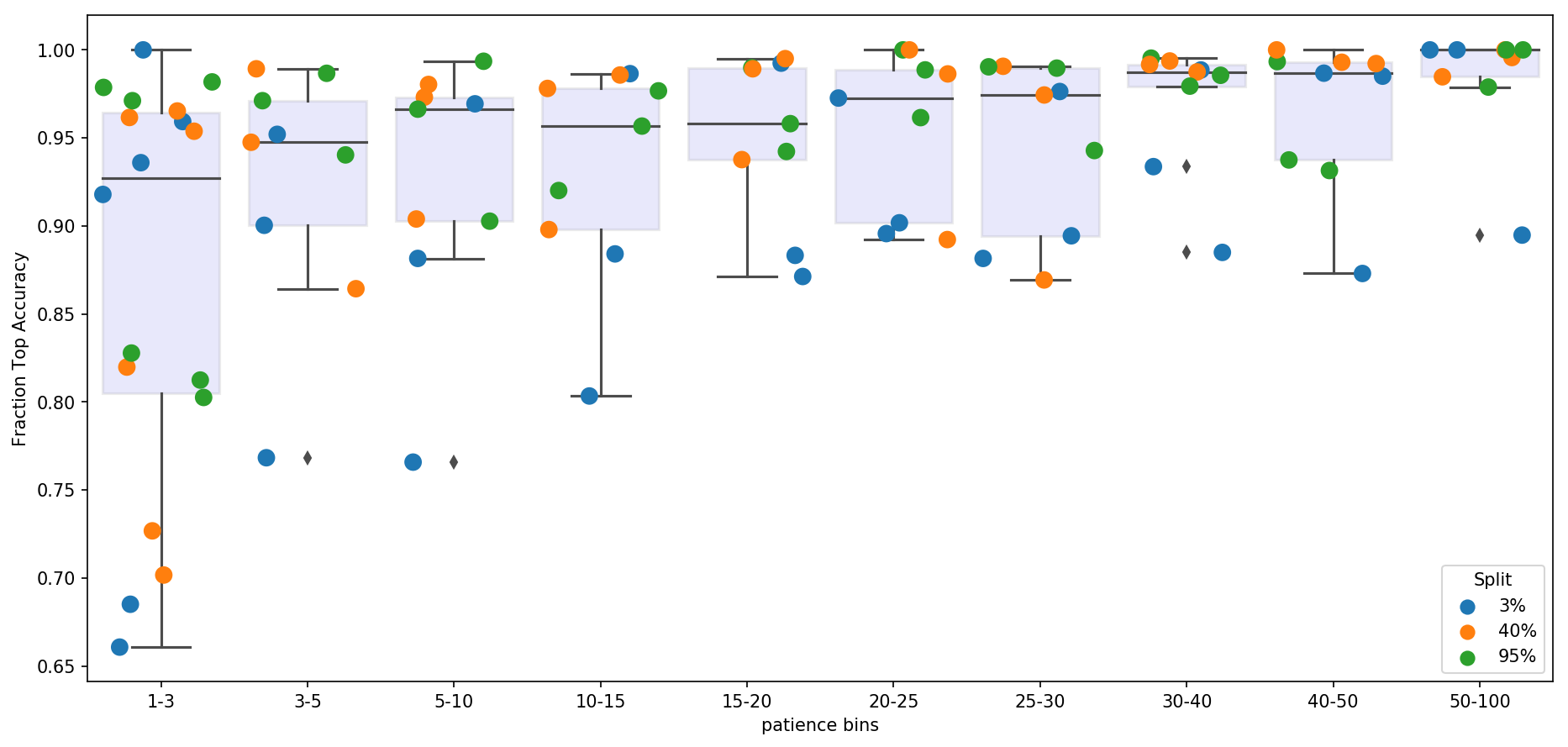
Our final results indicate that oveall accuracy of embeddings is a function of dataset size and n_epochs_without_progress. However, only marginal gain in performance is achieved when n_epochs_without_progress>20. For large datasets (n_observations>10000), n_epochs_without_progress between 3 and 5 comes to within 85% of optimal classification accuracy.

`model`¶

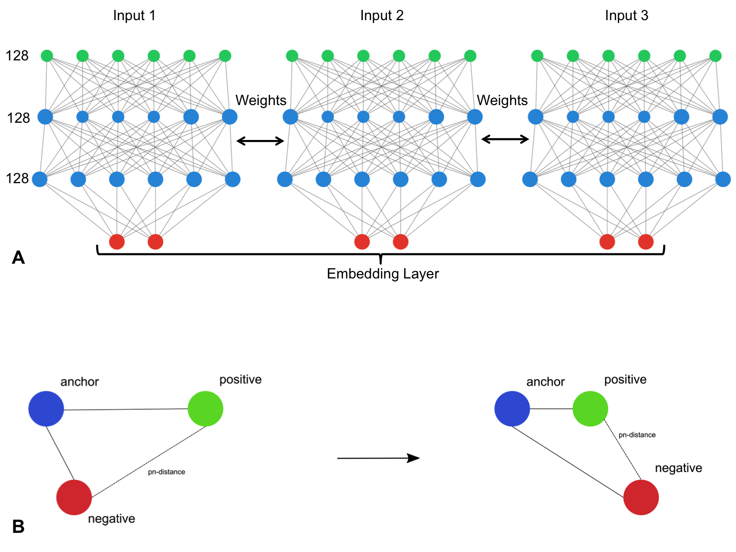
The model hyperparameter is a powerful way for ivis to handle complex non-linear feature-spaces. It refers to a trainable neural network that learns to minimise a triplet loss loss function. Structure-preserving dimensionality reduction is achieved by creating three replicates of the baseline architecture and assembling these replicates using a siamese neural network (SNNs). SNNs are a class of neural network that employ a unique architecture to naturally rank similarity between inputs. The ivis SNN consists of three identical base networks; each base network is followed by a final embedding layer. The size of the embedding layer reflects the desired dimensionality of outputs.

model parameter is defined using a keras model. This flexibility allows ivis to be trained using complex architectures and patterns, including convolutions. Out of the box, ivis supports three styles of baseline architectures - szubert, hinton, and maaten. This can be passed as string values to the model parameter.

‘szubert’¶

The szubert network has three dense layers of 128 neurons followed by a final embedding layer (128-128-128). The size of the embedding layer reflects the desired dimensionality of outputs. The layers preceding the embedding layer use the SELU activation function, which gives the network a self-normalizing property. The weights for these layers are randomly initialized with the LeCun normal distribution. The embedding layers use a linear activation and have their weights initialized using Glorot’s uniform distribution.

‘hinton’¶

The hinton network has three dense layers (2000-1000-500) followed by a final embedding layer. The size of the embedding layer reflects the desired dimensionality of outputs. The layers preceding the embedding layer use the SELU activation function. The weights for these layers are randomly initialized with the LeCun normal distribution. The embedding layers use a linear activation and have their weights initialized using Glorot’s uniform distribution.

‘maaten’¶

The maaten network has three dense layers (500-500-2000) followed by a final embedding layer. The size of the embedding layer reflects the desired dimensionality of outputs. The layers preceding the embedding layer use the SELU activation function. The weights for these layers are randomly initialized with the LeCun normal distribution. The embedding layers use a linear activation and have their weights initialized using Glorot’s uniform distribution.

Let’s examine each architectural option in greater detail:

architecture = ['szubert', 'hinton', 'maaten']
embeddings = {}
for a in architecture:
    ivis = Ivis(k=150).fit(X_poly)
    embeddings[a] = ivis.transform(X_poly)

fig, axs = plt.subplots(1, 3, figsize=(15, 4), facecolor='w', edgecolor='k')
fig.subplots_adjust(hspace = 0.3, wspace = 0.2)

axs = axs.ravel()
for i, nn in enumerate(architecture):
    xy=embeddings[nn]
    axs[i].scatter(xy[:, 0], xy[:, 1], s = 0.1, c = y)
    axs[i].set_title(nn)

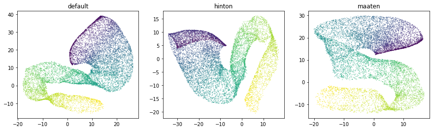
Selecting an appropriate baseline architecture is a data-driven task. Three unique architectures that are shipped with ivis perform consistently well across a wide array of tasks. A general rule of thumb in our own experiments is to use the szubert network for computationally-intensive processing on large datasets (>1 million observations) and select maaten architecture for smaller real-world datasets.

Custom backbone¶

Ivis also supports construction of arbitrary headless models, which can be helpful when dealing with multi-dimensional datasets such as images or text.

from tf.keras.applications.inception_v3 import InceptionV3

base_model = InceptionV3(include_top=False, pooling='avg')
ivis = Ivis(model=base_model)
ivis.fit()