Using ivis for Dimensionality Reduction of Single Cell Experiments
This example will demonstrate how ivis can be used to visualise
single cell experiments. Data import, preprocessing and normalisation
are handled by the Scanpy module.
The data that will be used in this example consists of 3,000 PBMCs from a
healthy donor and is freely available from 10x Genomics. Now, let’s
download the data and get started.
mkdir data
wget http://cf.10xgenomics.com/samples/cell-exp/1.1.0/pbmc3k/pbmc3k_filtered_gene_bc_matrices.tar.gz -O data/pbmc3k_filtered_gene_bc_matrices.tar.gz
cd data; tar -xzf pbmc3k_filtered_gene_bc_matrices.tar.gz
import numpy as np
import pandas as pd
import scanpy as sc

sc.settings.verbosity = 3
sc.logging.print_versions()
results_file = './write/pbmc3k.h5ad'

adata = sc.read_10x_mtx(
    './data/filtered_gene_bc_matrices/hg19/',  # the directory with the `.mtx` file
    var_names='gene_symbols',                  # use gene symbols for the variable names (variables-axis index)
    cache=True)                                # write a cache file for faster subsequent reading
We can now carry out basic filtering and handling of mitochondrial genes:
adata.var_names_make_unique()
sc.pp.filter_cells(adata, min_genes=200)
sc.pp.filter_genes(adata, min_cells=3)

mito_genes = adata.var_names.str.startswith('MT-')
# for each cell compute fraction of counts in mito genes vs. all genes
# the `.A1` is only necessary as X is sparse (to transform to a dense array after summing)
adata.obs['percent_mito'] = np.sum(
    adata[:, mito_genes].X, axis=1).A1 / np.sum(adata.X, axis=1).A1
# add the total counts per cell as observations-annotation to adata
adata.obs['n_counts'] = adata.X.sum(axis=1).A1

adata = adata[adata.obs['n_genes'] < 2500, :]
adata = adata[adata.obs['percent_mito'] < 0.05, :]
Let’s normalise the data and apply log-transformation:
sc.pp.normalize_per_cell(adata, counts_per_cell_after=1e4)
sc.pp.log1p(adata)
adata.raw = adata
Identify highly-variable genes and do the filtering:
sc.pp.highly_variable_genes(adata, min_mean=0.0125, max_mean=3, min_disp=0.5)

adata = adata[:, adata.var['highly_variable']]

sc.pp.regress_out(adata, ['n_counts', 'percent_mito'])
It’s recommended to apply PCA-transformation of normalised data - this step tends to denoise the data.
sc.pp.scale(adata, max_value=10)
sc.tl.pca(adata, svd_solver='arpack')
Reducing Dimensionality Using ivis
import matplotlib.pyplot as plt
from ivis import Ivis
For most single cell datasets, the following hyperparameters can be used:
k=15model='maaten'n_epochs_without_progress=5
Note
Keep in mind that this is a very small experiment (<3000 observations) and there are plenty of fast and accurate algorithm designed for these kinds of datasets e.g. UMAP. However, if you have >250,000 cells, ivis considerably outperforms state-of-the-art both in speed and accuracy of embeddings. See our timings benchmarks for more information on this.
X = adata.obsm['X_pca']

ivis = Ivis(k=15, model='maaten', n_epochs_without_progress=5)
ivis.fit(X)
embeddings = ivis.transform(X)
Finally, let’s visualise our embeddings, coloured by the CST3 gene!
fill = adata.X[:, adata.var.gene_ids.index=='CST3']
fill = fill.reshape((X.shape[0], ))
plt.figure(figsize=(6, 4), dpi=150)
sc = plt.scatter(x=embeddings[:, 0], y=embeddings[:, 1], c=fill, s=5)
plt.xlabel('ivis 1')
plt.ylabel('ivis 2')
plt.title('CST3')
plt.colorbar(sc)
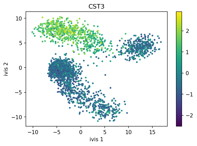
ivis effectively captured three distinct cellular populations in this small dataset. Note that ivis is an “honest” algorithm and distances between observations are meaningful. Our benchmarks show that ivis is ~10% better at preserving local and global distances in low-dimensional space than comparable state-of-the-art algorithms. Additionally, ivis is robust against noise and outliers, ulike t-SNE, which tends to group random noise into well-defined clusters that can be potentially misleading.