Metric Learning with Application to Supervised Anomaly Detection¶

Introduction¶

Metric Learning¶

Metric Learning is a machine learning task that aims to learn a distance function over a set of observations. This can be useful in a number of applications, including clustering, face identification, and recommendation systems.

ivis was developed to address this task using concepts of the Siamese Neural Networks. In this example, we will demonstrate that Metric Learning using ivis can effectively deal with class imbalance, yielding features resulting in state-of-the-art classification performance.

Supervised Dimensionality Reduction¶

ivis is able to make use of any provided class labels to perform supervised dimensionality reduction. Supervised embeddings combine the distance-based characteristics of the unsupervised ivis algorithm with clear class boundaries between the class categories. This is achieved by simultaneously minimising the tripplet loss and softmax loss functions. The resulting embeddings encode relevant class-specific information into lower dimensional space. It is possible to control the relative importance ivis places on class labels when training in supervised mode with the supervision_weight parameter. This variable should be a float between 0.0 to 1.0, with higher values resulting in classification affecting the training process more, and smaller values resulting in it impacting the training less. By default, the parameter is set to 0.5. Increasing it to 0.8 will result in more cleanly separated classes.

Results¶

Data Selection¶

In this example we will make use of the Credit Card Fraud Dataset. The datasets contains transactions made by credit cards in September 2013 by european cardholders. This dataset presents transactions that occurred in two days, where we have 492 frauds out of 284,807 transactions. The dataset is highly unbalanced, the positive class (frauds) account for 0.172% of all transactions. Traditional supervised classification approaches would typically balance the training dataset either by over-sampling the minority class or down-sampling the majority class. Here, we investigate how ivis handles class embalance.

Data Preparation¶

import pandas as pd
import matplotlib.pyplot as plt

from sklearn.preprocessing import StandardScaler, MinMaxScaler
from sklearn.model_selection import train_test_split
from sklearn.metrics import confusion_matrix, average_precision_score, roc_auc_score, classification_report
from sklearn.linear_model import LogisticRegression

from ivis import Ivis

data = pd.read_csv('../input/creditcard.csv')
Y = data['Class']

The Credit Card Fraud dataset is highly skewed, consisting of 492 frauds in a total of 284,807 observations (0.17% fraud cases). The features consist of numerical values from the 28 ‘Principal Component Analysis (PCA)’ transformed features, as well as Time and Amount of a transaction.

In this analysis we will train ivis algorithm using a 5% stratified subsample of the dataset. Our previous experiments have shown that ivis can yield >90% accurate embeddings using just 1% of the total data.

train_X, test_X, train_Y, test_Y = train_test_split(data, Y, stratify=Y,
                                                    test_size=0.95, random_state=1234)

Next, because ivis will learn a distance over observations, scaling must be applied to features. Additionally, transforming the data to a range [0, 1] allows the neural network to extract more meaningful features.

standard_scaler = StandardScaler().fit(train_X[['Time', 'Amount']])
train_X.loc[:, ['Time', 'Amount']] = standard_scaler.transform(train_X[['Time', 'Amount']])
test_X.loc[:, ['Time', 'Amount']] = standard_scaler.transform(test_X[['Time', 'Amount']])

minmax_scaler = MinMaxScaler().fit(train_X)
train_X = minmax_scaler.transform(train_X)
test_X = minmax_scaler.transform(test_X)

Dimensionality Reduction¶

Now, we can run ivis using default hyperparameters for supervised embedding problems:

ivis = Ivis(embedding_dims=2, model='maaten',
            k=15, n_epochs_without_progress=5,
            supervision_weight=0.80,
            verbose=0)
ivis.fit(train_X, train_Y.values)

ivis.save_model('ivis-supervised-fraud')

Finally, let’s embed the training set and extrapolate learnt embeddings to the testing set.

train_embeddings = ivis.transform(train_X)
test_embeddings = ivis.transform(test_X)

Visualisations¶

fig, ax = plt.subplots(1, 2, figsize=(17, 7), dpi=200)
ax[0].scatter(x=train_embeddings[:, 0], y=train_embeddings[:, 1], c=train_Y, s=3, cmap='RdYlBu_r')
ax[0].set_xlabel('ivis 1')
ax[0].set_ylabel('ivis 2')
ax[0].set_title('Training Set')

ax[1].scatter(x=test_embeddings[:, 0], y=test_embeddings[:, 1], c=test_Y, s=3, cmap='RdYlBu_r')
ax[1].set_xlabel('ivis 1')
ax[1].set_ylabel('ivis 2')
ax[1].set_title('Testing Set')

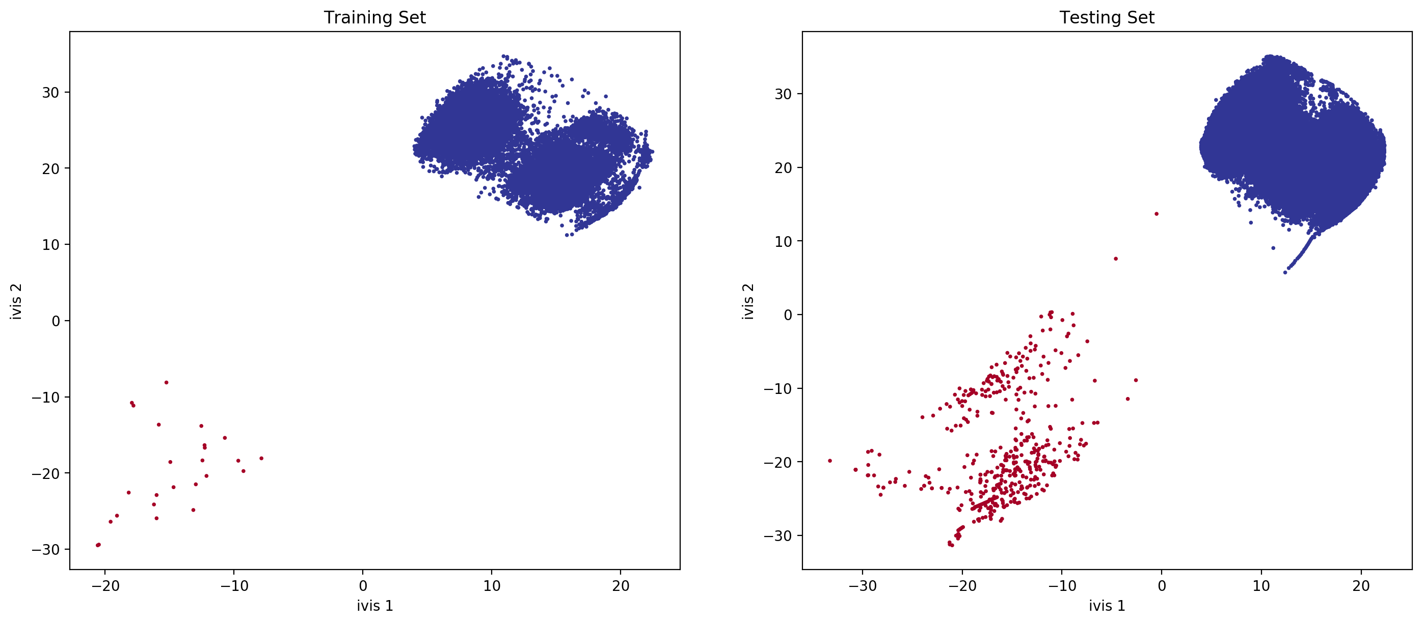
With anomalies being shown in red, we can see that ivis:

Effectively learnt embeddings in an unbalanced dataset.
Succesfully extrapolated learnt metrics to a testing subset.

Linear Classifier¶

We can train a simple linear classifier to assess how well ivis learned the class representations.

clf = LogisticRegression(solver="lbfgs").fit(train_embeddings, train_Y)

labels = clf.predict(test_embeddings)
proba = clf.predict_proba(test_embeddings)

print(classification_report(test_Y, labels))

print('Confusion Matrix')
print(confusion_matrix(test_Y, labels))
print('Average Precision: '+str(average_precision_score(test_Y, proba[:, 1])))
print('ROC AUC: '+str(roc_auc_score(test_Y, labels)))

              precision    recall  f1-score   support

           0       1.00      1.00      1.00    270100
           1       1.00      0.99      1.00       467

    accuracy                           1.00    270567
   macro avg       1.00      1.00      1.00    270567
weighted avg       1.00      1.00      1.00    270567

Confusion Matrix
[[270100      0]
[     3    464]]
Average Precision: 0.9978643591710002
ROC AUC: 0.9967880085653105

Conclusions¶

ivis effectively learns a distance metric over an unbalanced dataset. The resulting feature set can be used with a simple linear model classifier to achieve state-of-the-art performance on a classification task.